Diffusion Model
Research Notes: Diffusion model
Welcome to my personal study survey. This page documents my reading history, project implementations, and knowledge tracking in DM.
1. The Evolution of Diffusion Models
Pre-2020: Theoretical Foundations
- [ICML 2015] Deep Unsupervised Learning using Nonequilibrium Thermodynamics [Paper]
- [NeurIPS 2019] Generative Modeling by Estimating Gradients of the Data Distribution (NCSN) [Paper] [Code]
summary: score matching的开始.
2020: The Breakthrough
- [NeurIPS 2020] Denoising Diffusion Probabilistic Models (DDPM) [Paper] [Code] ⭐⭐⭐⭐⭐
summary: Diffusion model 的开山之作,forward(加噪)+reverse(去噪) process,用U-net预测 $\varepsilon$ , \(\mathbb{L}=\mathbb{E}_{t, x_0, \epsilon} \left[ \| \epsilon - \epsilon_\theta(x_t, t) \|^2 \right]\) ,但缺点是马尔科夫链采样慢,同时在像素空间做预测,计算资源消耗大.
- [ICLR 2021] Denoising Diffusion Implicit Models (DDIM) [Paper] [Code] ⭐⭐⭐⭐
summary: 从工程学角度出发,敏锐观察到:将reverse公式方差设成0,reverse process变成非马尔科夫链的ODE,实现跳步采样,但是依旧未实现一步采样.
2021: Guidance Mechanisms
- [NeurIPS 2021] Diffusion Models Beat GANs on Image Synthesis (Classifier Guidance) [Paper] [Code] ⭐⭐⭐
- [NeurIPS 2022] Classifier-Free Diffusion Guidance (CFG) [Paper] ⭐⭐⭐⭐
summary: 同时训练有condition和无condition情况,并在推理时利用 Guidance Scale 放大两者预测噪声的差异.
\[\hat{\epsilon}_{\theta}(x_t, c) = \epsilon_{\theta}(x_t, \varnothing) + w \cdot (\epsilon_{\theta}(x_t, c) - \epsilon_{\theta}(x_t, \varnothing))\]创新点: 类似 (prompt/condition) dropout 设计,实现生成质量与多样性的平衡.
2022: Latent Space & Controllability
- [CVPR 2022] High-Resolution Image Synthesis with Latent Diffusion Models (Stable Diffusion) [Paper] [Code] ⭐⭐⭐⭐⭐️
summary: SDM是当前扩散模型的主流架构,同时引入了VAE做latent space,CFG做无分类器,cross-attention 的U-net,CLIP做条件特征向量提取.
- [ICCV 2023] Adding Conditional Control to Text-to-Image Diffusion Models (ControlNet) [Paper] [Code] ⭐⭐⭐⭐
summary: 在冻结 SDM 参数基础上,复制其 Encoder 和 Middle Block 作为可训练分支进行微调;然后将 特征 经过该copy部分的block计算后,通过 Zero Convolution 注入到原冻结模型的 Skip Connections 上并一同传入 Decoder。
核心创新点: 类似于 ResNet 的残差机制,初始化时零卷积等效于零,宁可学不到特征也绝不传入错误的梯度参数,完美保护了原模型强大的生成能力。
2023-Present(2026): Efficiency & Flow Matching
- [ICML 2023] Consistency Models [Paper] [Code] ⭐⭐⭐⭐
summary: 从数学理论角度推导,对数学理论要求较高,实现了两种训练算法,很有意思.
- [ICLR 2023] Flow Matching for Generative Modeling [Paper]
2. Literature Review
Foundations of Generative Models
- [ICLR 2014] Auto-Encoding Variational Bayes [Paper] ⭐⭐⭐⭐
Core Concept: This paper proposes the Variational Autoencoder (VAE), a foundational generative model.
How it Works: It compresses input images into a probability distribution instead of fixed numbers. ( ELBO )
Major Innovation: The paper introduces the Reparameterization Trick , which allows the network to calculate gradients through random sampling. ($z = \mu + \sigma \odot \epsilon$, Instead of sampling $z$ directly, we introduce an independent noise variable $\epsilon$ sampled from a standard normal distribution)
Final Outcome: This makes end-to-end training possible, allowing the model to generate entirely new images.
- [ICML 2015] Deep Unsupervised Learning using Nonequilibrium Thermodynamics [Paper] ⭐⭐⭐⭐
Core Diffusion Models
Core Paradigm: DDPM frames generative modeling as a two-stage Markov chain process: a fixed forward diffusion phase that systematically destroys data, and a learned reverse denoising phase that reconstructs data from noise.
Forward Process (Diffusion): This is a fixed, parameterized Markov chain that incrementally adds isotropic Gaussian noise to the original data over $T$ steps, dictated by a predefined variance schedule. Utilizing the reparameterization trick , the framework allows for the efficient sampling of the corrupted image $x_t$ at any arbitrary timestep $t$ in a single closed-form calculation.
Reverse Process (Denoising): This learnable Markov chain is parameterized by a deep neural network, typically utilizing a U-Net architecture enhanced with spatial attention. Starting from pure isotropic Gaussian noise $x_T$, the network iteratively predicts and subtracts the noise at each discrete step, progressively restoring the intricate high-dimensional structures to generate a coherent image $x_0$.
Optimization Objective: The mathematically intensive optimization of the Evidence Lower Bound (ELBO) is elegantly simplified into a highly stable surrogate loss. The neural network is trained using a Mean Squared Error (MSE) objective to predict the exact noise tensor $\epsilon$ injected during the forward process, purposefully avoiding the direct prediction of the original image or the distribution’s mean.
Mathematical Formulation and Core Equations
Forward Process: Gradually adding noise through a Markov chain, the single-step conditional distribution is:
\[q(x_t | x_{t-1}) = \mathcal{N}(x_t; \sqrt{1 - \beta_t} x_{t-1}, \beta_t \mathbf{I})\]Utilizing the reparameterization trick, the closed-form sampling at any arbitrary timestep $t$ can be directly obtained from $x_0$ (where $\bar{\alpha}_t$ is the cumulative product parameter):
\[q(x_t | x_0) = \mathcal{N}(x_t; \sqrt{\bar{\alpha}_t} x_0, (1 - \bar{\alpha}_t) \mathbf{I})\]Reverse Process: The denoising process parameterized by a neural network is defined as:
\[p_\theta(x_{t-1} | x_t) = \mathcal{N}(x_{t-1}; \mu_\theta(x_t, t), \Sigma_\theta(x_t, t))\]Simplified Optimization Objective (Simplified Loss): Discarding the complex ELBO weighting, it directly optimizes the L2 distance between the predicted noise and the true injected noise:
\[L_{\text{simple}} = \mathbb{E}_{t, x_0, \epsilon} \left[ \| \epsilon - \epsilon_\theta(\sqrt{\bar{\alpha}_t} x_0 + \sqrt{1 - \bar{\alpha}_t} \epsilon, t) \|^2 \right]\]
def ddpm_training_step(x_0, t, unet):
    # 1. Generate standard Gaussian noise of the same size as the original image (corresponds to epsilon in the formula)
    noise = torch.randn_like(x_0)

    # 2. Retrieve the cumulative alpha parameter for the current timestep t from the predefined schedule
    sqrt_alpha_bar = sqrt_alphas_cumprod[t]
    sqrt_one_minus_alpha_bar = sqrt_one_minus_alphas_cumprod[t]

    # 3. Forward diffusion: directly calculate the noisy image x_t at any arbitrary timestep t using the closed-form formula
    x_t = sqrt_alpha_bar * x_0 + sqrt_one_minus_alpha_bar * noise

    # 4. Reverse denoising: U-Net predicts the added noise epsilon_theta
    predicted_noise = unet(x_t, t)

    # 5. Optimization objective: calculate the Mean Squared Error (MSE Loss) between the predicted noise and the true noise
    loss = F.mse_loss(predicted_noise, noise)

    return loss
Core Paradigm: DDIM generalizes the Markov chain forward process of DDPMs to non-Markovian processes . It achieves the exact same training objective (matching the marginal distributions) but fundamentally alters the sampling trajectory.
Accelerated Deterministic Sampling: Unlike DDPM, which strictly requires hundreds or thousands of sequential steps due to its stochastic Markov reliance, DDIM formulates a deterministic generative process . By removing the random noise injection during the reverse step, it can “jump” across multiple timesteps (sub-sequence sampling). This elegant mathematical reframing accelerates inference by 10x to 50x without requiring any model retraining .
Latent Space Interpolation & Invertibility: Because the DDIM reverse sampling process is deterministic (when the stochastic variance parameter is set to zero), it creates a meaningful, invertible mapping between the initial Gaussian noise vector and the final generated image. This unlocks the ability to perform smooth semantic interpolations in the latent noise space—a feature that was practically impossible with the highly stochastic DDPMs.
Mathematical Formulation and Core Equation
DDIM generalizes the generative process by introducing a variance parameter $\sigma_t$ to control the stochasticity of the sampling process. The reverse sampling formula from timestep $t$ to $t-1$ is defined as:
\[x_{t-1} = \sqrt{\alpha_{t-1}} \underbrace{\left( \frac{x_t - \sqrt{1 - \alpha_t} \epsilon_\theta(x_t, t)}{\sqrt{\alpha_t}} \right)}_{\text{predicted } x_0} + \underbrace{\sqrt{1 - \alpha_{t-1} - \sigma_t^2} \cdot \epsilon_\theta(x_t, t)}_{x_0 \text{ direction pointing to } x_t} + \underbrace{\sigma_t \epsilon}_{\text{random noise}}\]Core Parameter Analysis:
- When $\sigma_t = \sqrt{\frac{1 - \alpha_{t-1}}{1 - \alpha_t}} \sqrt{1 - \frac{\alpha_t}{\alpha_{t-1}}}$, the process is equivalent to the highly stochastic DDPM (Markov process).
- When $\sigma_t = 0$, the random noise term in the formula completely disappears. At this point, the reverse process becomes completely deterministic , which is the essence of “DDIM”, and also the mathematical foundation that enables its step-jumping acceleration (e.g., skipping multiple $t$ for direct sampling).
def ddim_sample_step(x_t, t, t_prev, unet):#prev=previous
    # 1. Pass in the current latent variable and timestep, predict the noise epsilon for the current timestep via U-Net
    noise_pred = unet(x_t, t)

    # 2. Retrieve the corresponding cumulative alpha product from the predefined schedule
    alpha_t = alphas_cumprod[t]
    alpha_t_prev = alphas_cumprod[t_prev]

    # 3. Core calculation: derive the predicted value of the clean image x_0 based on the formula
    pred_x0 = (x_t - torch.sqrt(1 - alpha_t) * noise_pred) / torch.sqrt(alpha_t)

    # 4. Core calculation: compute the direction term pointing to x_t (at this stage sigma_t = 0, no stochastic variance is added)
    dir_xt = torch.sqrt(1 - alpha_t_prev) * noise_pred

    # 5. Combine the two terms above to deterministically obtain the latent variable x_{t-1} for the previous timestep
    x_t_prev = torch.sqrt(alpha_t_prev) * pred_x0 + dir_xt

    return x_t_prev
- [NeurIPS 2022] Classifier-Free Diffusion Guidance (CFG) [Paper] ⭐⭐⭐⭐
Core Paradigm: CFG is a revolutionary technique that allows diffusion models to perform high-fidelity conditional generation (e.g., text-to-image) without the need to train a separate, noise-robust image classifier.
Architectural Mechanism (Joint Training): The diffusion model is jointly trained on both conditional and unconditional objectives. During training, the conditioning signal (such as a text prompt) is randomly dropped out (replaced with a null token) with a certain probability (e.g., 10% to 20%). This forces a single neural network to master both conditional generation and unconditional generation simultaneously.
Inference & Impact: During the reverse sampling process, the model calculates a vector pointing away from the unconditional prediction and towards the conditional prediction. By amplifying this directional vector with a guidance scale, it achieves a superior trade-off between sample fidelity and diversity. This elegant algebraic operation is the fundamental steering wheel for almost all modern multi-modal diffusion architectures.
def cfg_sampling_step(unet, latent_input, t, cond_emb, uncond_emb, guidance_scale):
    # 1. Duplicate latent input to compute unconditional and conditional predictions simultaneously
    latent_batched = torch.cat([latent_input, latent_input], dim=0)

    # 2. Concatenate unconditional (null) and conditional (prompt) context embeddings
    context_batched = torch.cat([uncond_emb, cond_emb], dim=0)

    # 3. Single U-Net forward pass to predict noise for both conditions
    noise_pred = unet(latent_batched, t, context=context_batched)

    # 4. Split the batched predictions back into unconditional and conditional tensors
    noise_pred_uncond, noise_pred_cond = noise_pred.chunk(2, dim=0)

    # 5. Apply Classifier-Free Guidance formula to extrapolate the conditional direction
    noise_guided = noise_pred_uncond + guidance_scale * (noise_pred_cond - noise_pred_uncond)

    return noise_guided
- [CVPR 2022] High-Resolution Image Synthesis with Latent Diffusion Models (Stable Diffusion) [Paper] [Code] ⭐⭐⭐⭐⭐
Core Paradigm: Latent Diffusion Models (LDMs) revolutionize the generative framework by shifting the computationally intensive diffusion process from the high-dimensional pixel space into a compressed, low-dimensional latent space, enabling highly efficient high-resolution image synthesis.
Forward Process (Diffusion in Latent Space): A pre-trained perceptual compression autoencoder transforms the original image into a condensed latent representation. The forward Markov chain then systematically injects isotropic Gaussian noise into this latent vector across discrete timesteps, following a fixed variance schedule, rather than corrupting the pixel-level image.
Reverse Process (Conditional Denoising): A highly specialized time-conditional U-Net, empowered by cross-attention mechanisms, iteratively removes noise from the corrupted latent vector. It seamlessly integrates multi-modal conditioning inputs (such as text prompts encoded by CLIP, or spatial layouts), guiding the reverse process to reconstruct specific representations. Finally, a dedicated decoder maps the clean latent vector back into the pixel space.
Optimization Objective: The training mathematically simplifies the complex variational lower bound into a straightforward latent-space objective. The neural network is optimized via Mean Squared Error (MSE) to predict the exact noise injected into the latent representation, drastically reducing computational overhead.
Impact and Multimodal Extension: By fundamentally decoupling the autoencoding compression phase from the generative diffusion phase, LDMs democratize high-fidelity synthesis. It serves as the core engine for Stable Diffusion, profoundly advancing computer vision and dominating modern text-to-image multi-modal systems.
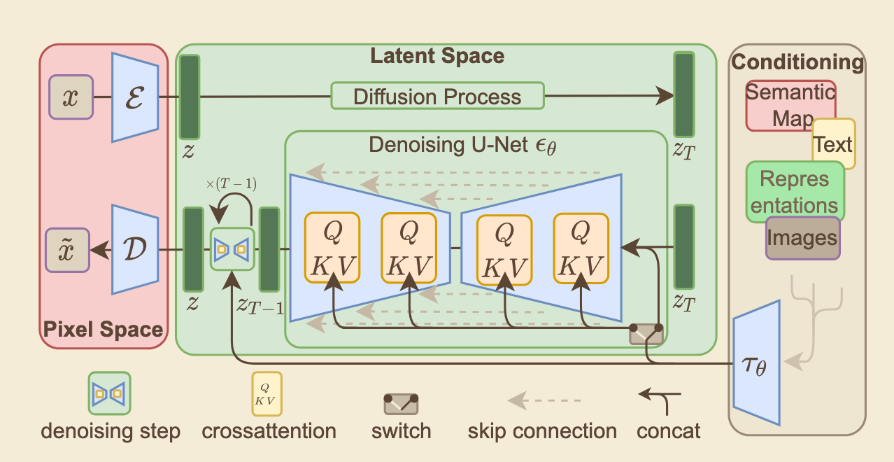
Architecture Overview: Stable Diffusion Model utilizing a pre-trained autoencoder and Cross-Attention conditioned U-Net .
def latent_train_loss(x_0, context):
    # Encode high-dimensional image to low-dimensional latent space
    z_0 = encoder(x_0)

    # Sample random timestep t
    t = torch.randint(1, T + 1, (z_0.shape[0],))

    # Generate standard Gaussian noise in latent space
    epsilon = torch.randn_like(z_0)

    # Add noise to latent representation z_0 to get corrupted z_t
    z_t = sqrt_alphas_cumprod[t] * z_0 + sqrt_one_minus_alphas_cumprod[t] * epsilon

    # Encode conditioning context (e.g., text prompt)
    c = context_encoder(context)

    # U-Net predicts the added noise conditioned on t and c
    predicted_noise = unet(z_t, t, context=c)

    # Calculate MSE loss between predicted and actual noise
    loss = F.mse_loss(predicted_noise, epsilon)

    return loss
- [ICCV 2023] Adding Conditional Control to Text-to-Image Diffusion Models (ControlNet) [Paper] [Code] ⭐⭐⭐⭐
Core Paradigm: ControlNet introduces an end-to-end neural network architecture designed to add fine-grained, spatial conditional control (such as Canny edges, depth maps, user scribbles, or human poses) to large, pre-trained text-to-image diffusion models without disrupting their foundational generative capabilities .
Architectural Mechanism (Structural Cloning): The framework freezes the parameters of the original pre-trained U-Net to prevent catastrophic forgetting. It then creates a trainable “clone” of the network’s encoding blocks . The spatial conditioning image is processed through this trainable copy to extract condition-specific feature maps .
Zero Convolutions: The trainable encoding branch connects back to the frozen decoding backbone via “zero convolutions” - 1x1 convolutional layers with weights and biases initialized to exactly zero . This ingenious initialization ensures that at the very first training step, the conditioning branch outputs zero , leaving the pre-trained model’s original behavior perfectly intact and stable before any gradient updates occur.
Optimization & Impact: By locking the massive generative backbone and only updating the cloned layers, ControlNet enables highly data-efficient and memory-efficient fine-tuning . It allows robust training on specialized tasks with datasets as small as a few thousand image-condition pairs , fundamentally solving the spatial controllability problem in generative AI workflows.
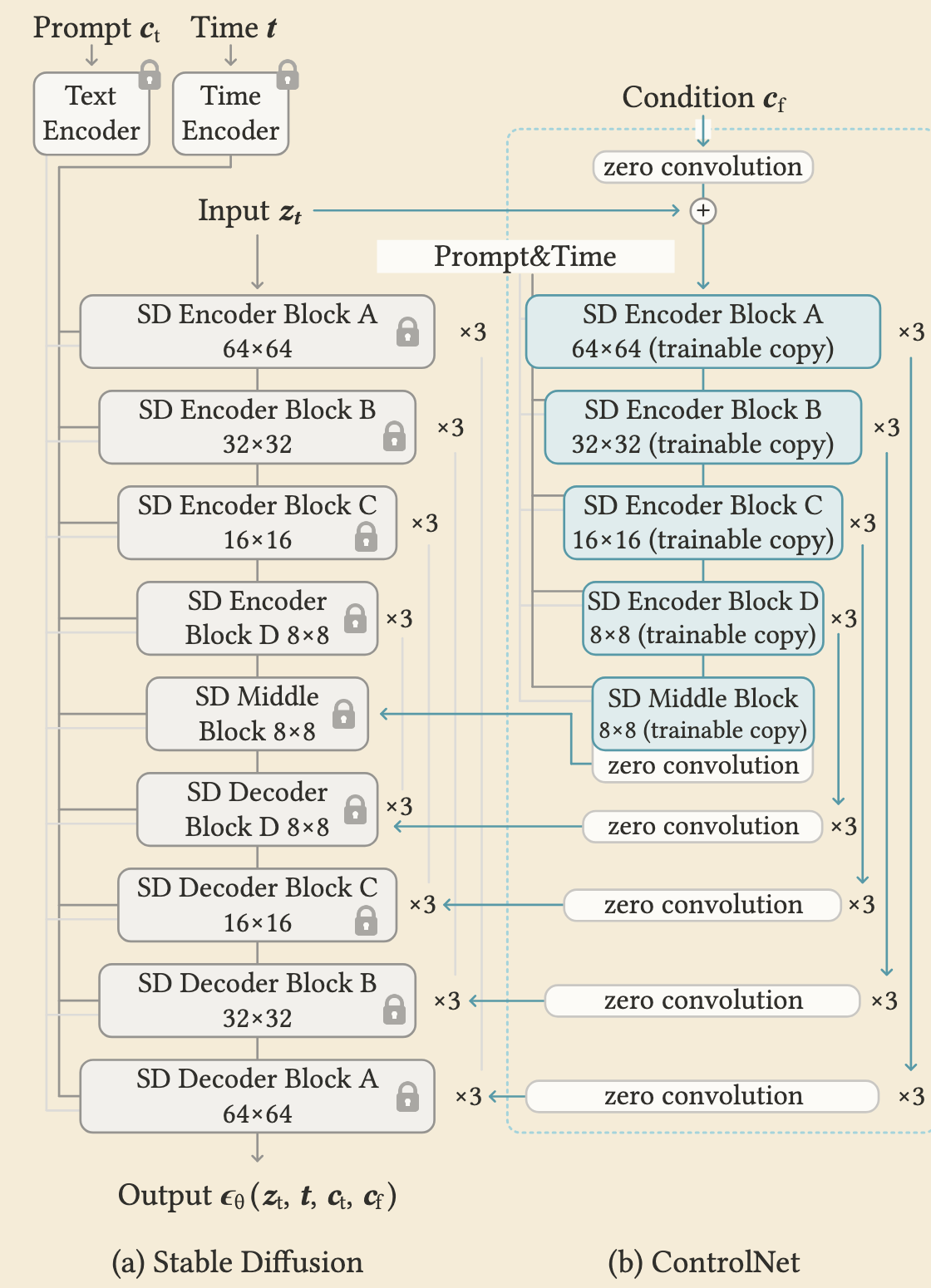
Stable Diffusion backbone (frozen) + trainable ControlNet copy with zero-conv feature injection.
def controlnet_forward(x_t, t, context, condition):
    # 1. Pass noisy latent (x_t) through the frozen SD encoder
    locked_features = frozen_encoder(x_t, t, context)

    # 2. Extract features from the spatial condition (e.g., edge map)
    condition_features = condition_encoder(condition)

    # 3. Pass through the trainable ControlNet copy
    # Condition is added to the noisy latent at the input level
    control_input = x_t + condition_features
    control_features = trainable_encoder(control_input, t, context)

    # 4. Apply Zero Convolutions (initialized to 0)
    guided_features = [zero_conv(f) for f, zero_conv in zip(control_features, zero_convs)]

    # 5. Add guided features into the frozen model's decoder connections
    output = frozen_decoder(locked_features, guided_features, t, context)

    return output
Core Paradigm: The paper challenges the modern standard of predicting noise ($\epsilon$-prediction) or velocity ($v$-prediction). Instead, it advocates for a return to first principles: predicting the clean data directly ($x$-prediction). Based on the Manifold Assumption, natural data lies on a low-dimensional manifold, while noise distributes across the full high-dimensional space. Thus, predicting clean images is fundamentally easier for neural networks.
Forward Process (High-Dimensional Pixel Space): Unlike Latent Diffusion Models that rely on pre-trained autoencoders to compress data, this approach operates directly on raw, high-dimensional pixel patches. The forward process incrementally adds noise to the data to create interpolations between the clean image and pure noise.
Reverse Process (Just Image Transformers-JiT): The reverse denoising process is driven by a surprisingly simple architecture named “Just image Transformers” (JiT). It is essentially a plain Vision Transformer (ViT) that processes large patches of pixels without requiring hierarchical designs, latent tokenizers, or self-supervised pre-training.
Optimization Objective: The network is strictly parameterized to predict the clean data ($x$), but the optimization is calculated using a flow-matching velocity loss ($v$-loss). The paper demonstrates that while predicting noise fails catastrophically in high-dimensional patch spaces, $x$-prediction succeeds elegantly even with under-capacity networks.
def jit_train_loss(x, t):
    # Sample random noise
    e = torch.randn_like(x)

    # Corrupt the image (forward process interpolation)
    z = t * x + (1 - t) * e

    # JiT network predicts the CLEAN data (x-prediction)
    x_pred = net(z, t)

    # Transform the x-prediction to velocity (v) space
    v_pred = (x_pred - z) / (1 - t)

    # Calculate the true velocity
    v = x - e

    # Output the L2 loss in v-space
    loss = l2_loss(v, v_pred)

    return loss
Medical Image Synthesis
- [ArXiv] MedDiff-FT: Data-Efficient Diffusion Model Fine-tuning with Structural Guidance for Controllable Medical Image Synthesis [Paper] [Code] ⭐⭐⭐⭐
Problem Statement
- Data Scarcity: The deep learning for medical image segmentation is severely limited by the lack of high-quality, annotated training data.
- Limitations of Diffusion Models: While diffusion models excel at synthetic data generation, they typically require large-scale datasets and struggle to generate the accurately paired image-mask datasets required for medical segmentation tasks.
Proposed Method (MedDiff-FT)
- Core Concept: The authors propose MedDiff-FT, a data-efficient and controllable framework that fine-tunes a foundation model (Stable Diffusion 1.5) to synthesize high-quality medical images with their corresponding structural masks.
Systematic Architecture
- Efficient Fine-Tuning (Training): The framework unfreezes the U-Net parameters and fine-tunes the model using very limited data (around 30 samples). It uses specialized text prompts to force the model to focus exclusively on learning the features of the lesion regions.
- Controllable Synthesis (Inference): During generation, the method uses a dynamic adaptive guiding mask alongside a background image. This spatially constrains the generation, ensuring the synthetic lesions are anatomically coherent and appear precisely where the mask dictates.
- Diversity Enhancement: To prevent mode collapse, the framework incorporates a lightweight, DDPM-based mask generator to create diverse structural shapes. It also utilizes a conditional image restorer to generate healthy, lesion-free tissue backgrounds.
- Quality Assessment & Post-processing: The system employs DINOv2 to calculate feature-space cosine similarity, automatically filtering out generated images that are of suboptimal quality. Finally, a morphological corrosion operation is applied to refine the annotation boundaries, making the mask fit the generated lesion better.
Experimental Results
- Performance: Evaluated across 5 datasets (covering skin, breast, and thyroid imaging) and 4 baseline architectures (like nnU-Net and Swin Transformer), the synthetic image-mask pairs improved segmentation Dice scores by an average of 1% to 3%.
- Efficiency: The training process is highly resource-efficient, taking under 30 minutes and consuming less than 24GB of memory.
- [ArXiv] SkinDualGen: Prompt-Driven Diffusion for Simultaneous Image-Mask Generation in Skin Lesions [Paper] ⭐⭐⭐
3. Empirical Implementations & Projects
MedDiff-FT: Data-Efficient Diffusion Model Fine-tuning
- Objective: Injecting custom visual concepts into pre-trained latent diffusion models.
- Code: [GitHub Repo Link]
- Notes: Overcoming catastrophic forgetting and learning rate tuning.
4. Concepts & Idea Pool
- Idea:
- Concept: